First-Order Reliability Method (FORM)

First-Order Reliability Method (FORM)#

This page gives an overview of the First-Order Reliability Method (FORM). It is an algorithm for solving the component reliability problem, which was first applied during Workshop 04. Once reading through this page, it may be useful to refer back to the solution for WS04, especially the graphical interpretation in the notebook.

A Linearized Solution#

The “FO” part of the algorithm name stands for “First Order” because the method is based on a linearized approximation (using a Taylor Series) of the limit-state function. This can be visualized in the figure below, where the

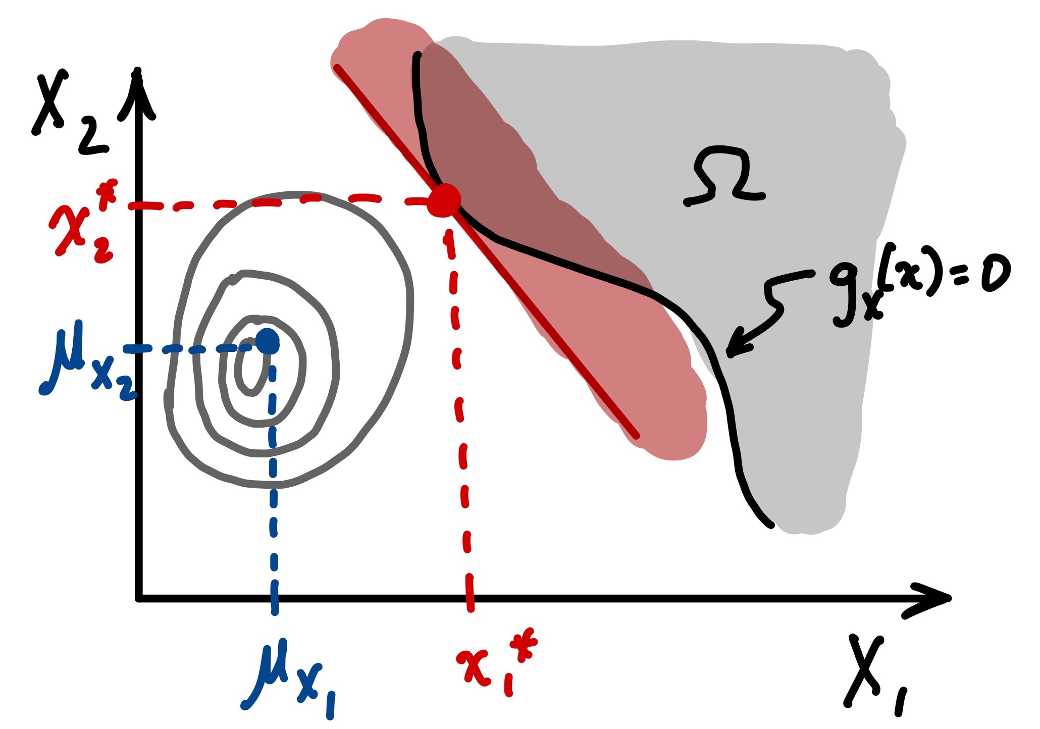
The contours illustrated in the figure are probability density. It is essential to recognize that the probability of interest (i.e., failure probability) is the volume underneath the shaded area and is found by integrating the probability density in the region of interest.

Design Point#

The design point is simply the expansion point of Taylor’s Series used in the linear approximation, of which there are infinite possible choices to select from. However, the FORM method uses a particular definition of the design point (also referred to as the Hasofer-Lind design point, after those who proposed it).

Specifically, the design point, \(x^*\), is:

A point on the limit-state surface such that \(g_X(x^*)=0\)
Of all the points on the limit-state surface, it is that which maximizes probability density \(f_X(x^*)\)

This is chosen for several reasons, the most important being that it produces a linearized limit-state function that will give the most suitable approximation of the failure probability, as well as producing insight into the problem of interest (i.e., the design variables and how they relate to the failure probability).

It is interesting to note that the design point also represents the shortest distance between the mean point of the probability density function and the limit-state surface. This will have a particularly important result when we transform the computations to the standard normal space, in the next section.

FORM is simply an algorithm that efficiently searches for the design point. It can be implemented with many optimization algorithms (e.g., in OpenTURNs we will use the Cobyla method).

Computations in Standard Normal Space#

Although we do not cover the approach here, the FORM calculations are actually being performed in the standard normal space. This makes the computations more feasible (we can use relatively simple distributions) as well as numerically more efficient. All random variables (including their multivariate distribution and the limit-state function) have been transformed to those with the Normal distribution of zero mean and variance of 1. The variables are also uncorrelated. This results in contours of probability density that are concentric circles, as illustrated in the figure below.

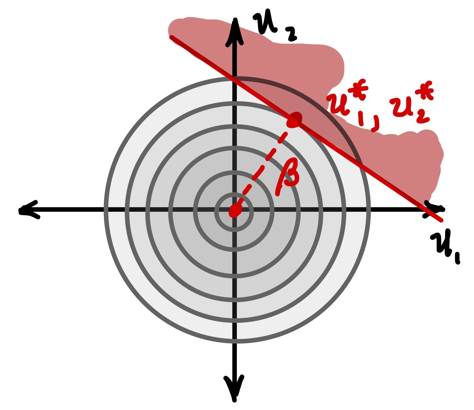
Note also that the distance between the mean point (origin) and the design point in the standard normal space (\(u^*\)) is the shortest distance to the limit-state surface. Because the limit-state is linearized, this distance is a normal vector (i.e., it is perpendicular).

Although this may seem like a strange approach, you have probably used the transformation before: it is in fact what you are doing when using a standard probability table for the Normal distribution! Typically, you convert the value of your random variable, \(X\), to another variable \(Z\), such that:

\[ z=\frac{x-\mu_X}{\sigma_X} \]

And the probability of \(Z\), the CDF \(F_Z(z)\), is found in the table. The key point here, relative to FORM, is that we performed the probability computation in the standard normal space (the \(Z\) variable). As illustrated in the figure above, we are using \(U\) to represent the multivariate standard normal variables.

Computing the Probability of Failure#

An interesting property of the standard normal space is that the mean of all random variables is at the origin, and the shortest distance to the limit-state surface is tangent to the linearized function. This distance, defined here as \(\beta\), makes the computation of failure probability straightforward using the CDF of the standard normal multivariate distribution, \(\Phi\):

\[ p_f = \Phi \big[-\beta\big] \]

Although this may seem complicated (due to the multivariate aspect), it is in fact no different than what you have done previously in the 1D standard normal case. Consider the figure below, which illustrates \(\beta\) as the “distance” between the mean and the point of interest (where we want to start our integral):

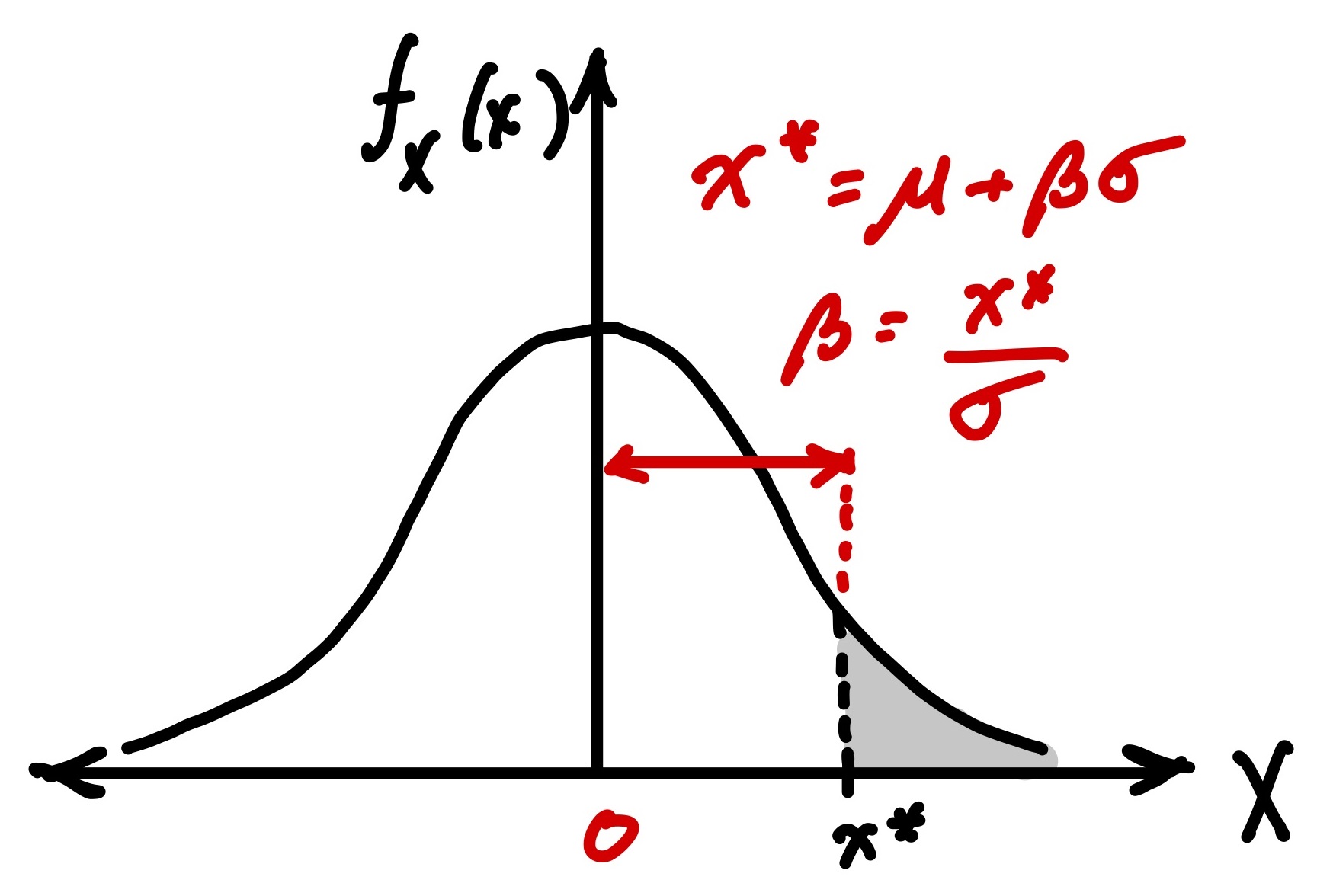
The value \(\beta\) is called the reliability index and is widely used in probabilistic design applications.

Relationship of \(\beta\) to \(\alpha\)#

From linear algebra, we can show that the distance, can be computed as the vector product:

\[ \beta = \alpha u^* \]

Where \(\alpha\) is a unit vector normal to the linearized limit state function:

\[ \alpha = -\frac{\nabla g_U(u^*)}{||\nabla g_U(u^*)||} \]

This is a vector of values, one for each of the \(n\) random variables:

\[ \alpha = \big[\alpha_1 \,\, \alpha_2 \,\, + \, \ldots \, + \,\, \alpha_n\big] \]

Importance Factors, \(\alpha\)#

The derivation of \(\alpha\) is outside the scope of our work, but it is important to recognize that it is found from the gradient of the limit-state function, which means it can be interpreted as a sensitivity. In addition, as it is computed in the standard normal space, which is transformed using the distributions of \(X\), it also incorporates the uncertainty of the random variables. As such, the \(\alpha\) values give useful insight into the component reliability problem:

It is a unit vector, so the sum of all values is 1
The magnitude of each element indicates the relative importance of the random variable towards the probability of failure
The sign indicates how the random variable acts on the function (negative values act as loads, positive values act as resistances)

Note that the interpretation of \(\alpha\) is straightforward, but one should remember that it is based on a linearized limit-state function with the design point as an expansion point. Results may be different in other regions of the failure domain, especially when high-dimensionality problems are considered (e.g., many random variables). This is why the term “act as a resistance/load” is used: for complex problems the random variables may change their behavior.

Computing \(\alpha\) Using OpenTURNs#

Note also that in reliability software there is no consistent definition of importance factors, although many use the notation \(\alpha\). For our purposes, the OpenTURNs package is a very useful tool, but their definition of \(\alpha\) is not that useful (it does not provide load/resistance information). The following code will produce the importance factors described above, once a multivariate distribution and limit-state function are defined (inputDistribution and myfunction) and a FORM result is obtained (result):

u_star = result.getStandardSpaceDesignPoint()
inverseTransform = inputDistribution.getInverseIsoProbabilisticTransformation()
failureBoundaryStandardSpace = ot.ComposedFunction(myfunction, inverseTransform)
du0 = failureBoundaryStandardSpace.getGradient().gradient(u_star)
g_grad = np.array(du0).transpose()[0]
alpha = -g_grad/np.linalg.norm(g_grad)
print('alpha = ')
[print(f'  {i:6.3f}') for i in alpha]

Essential Results of a FORM Analysis#

In summary, there are several key results from a FORM analysis that can help interpret the component reliability problem:

The reliability index allows straightforward computation of the failure probability: \(p_f=\Phi\big[-\beta\big]\)
The design point is the point on the limit-state surface that has the highest probability density (a proxy for highest probability of being the actual condition if failure occurs). In the original space and standard normal space it is represented as \(x^*\) and \(u^*\), respectively
The importance factors, \(\alpha\) indicates the relative importance of each random variable to the failure probability and includes information about the mechanical response of the limit-state function (i.e., the partial derivatives) as well as the uncertainty of the random variable (via the probability distribution).