Assignment 1

Introduction

In this assignment, we consider the behaviour of a soil layer which is subject to loading applied at the top. As shown in Figure 1, the load consists of a (temporary) soil body of very large size (in x and y directions), which allows to assume that there is no change in loading conditions in the horizontal directions, and neither in the response. Therefore, a 1‐dimensional model will suffice to predict the response of the soil layer, with only the z direction represented.

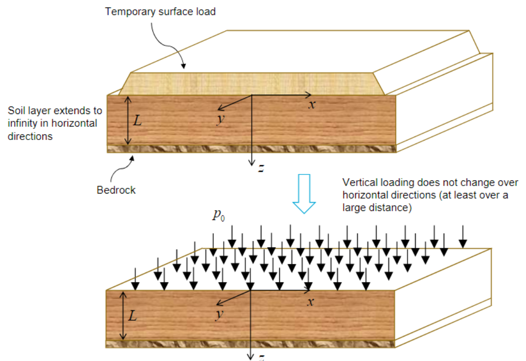
Fig. 1 Figure1

It is noted that plane‐strain condition applies (see Lecture 3). Due to the invariance of the load and of the structure, however, not only the strains in the \(y\) direction are zero, but also the ones in the \(x\) direction. This situation is referred to as uni‐axial strain.

The soil layer is characterized by constant material properties \(\rho\), \(E\), and \(\nu\), which are the mass density, the Young’s modulus and the Poisson’s ratio, respectively. The self‐weight of the layer is initially neglected, but it is accounted for in question 11. The thickness of the layer is denoted as L.

We assume that the soil layer rests on a bedrock (initially rigid, later on flexible), which prevents or elastically restrains displacements at the bottom of the layer. The magnitude of the loading (i.e., vertical stress) at the surface is denoted as \(p_0\)​.

Question 1

First the equation of motion governing the behaviour of the soil layer has to be determined as well as the boundary conditions.

Model answer

In general, the following stress-strain relations hold true for a plane strain situation:

• Zero strains in \(y\) direction (see Lecture 3 slide 6);

• Don’t use plane stress situation because you don’t know if there are no forces in y-direction in the soil. We only have information about the stresses (see introduction).

\[\begin{split} \begin{bmatrix} \sigma_{xx}\\ \sigma_{yy}\\ \sigma_{zz} \end{bmatrix} =\frac{E}{(1+\nu)(1-2\nu)} \begin{bmatrix} 1-\nu &\nu &0 \\ \nu &1-\nu &0 \\ 0 &0 &1-2\nu \end{bmatrix} \begin{bmatrix} \varepsilon_{xx}\\ \varepsilon_{zz}\\ \varepsilon_{xz} \end{bmatrix} \end{split}\]

In the specific situation of the current assignment, \(\varepsilon_{xx}\), \(\varepsilon_{xz}\)​ are zero as well (see Introduction).

Question 2

Question 3

Model answer

Due to the strain components in \(x\) and \(y\) directions being zero, the only nonzero stresses are \(\sigma_{xx}\), \(\sigma_{yy}\), \(\sigma_{zz}\)​ (see stiffness matrix where the other sigma’s are 0 because the strains are 0). Due to symmetry considerations and the absence of body forces in horizontal direction \(f_x=f_y=0\) (see figure in Introduction), there are no displacements in horizontal directions: \(u_x=u_y=0\).

Schematise the soil layer as a bar. These are the linearized momentum equations

\[\begin{split} \rho\frac{\partial^2 u_x}{\partial t^2}=\frac{\partial\sigma_{xx}}{\partial_x}+\frac{\partial\sigma_{yx}}{\partial_y}+\frac{\partial\sigma_{zx}}{\partial_z}+f_x\\ \rho\frac{\partial^2 u_y}{\partial t^2}=\frac{\partial\sigma_{xy}}{\partial_x}+\frac{\partial\sigma_{yy}}{\partial_y}+\frac{\partial\sigma_{zy}}{\partial_z}+f_y\\ \rho\frac{\partial^2 u_z}{\partial t^2}=\frac{\partial\sigma_{xz}}{\partial_x}+\frac{\partial\sigma_{yz}}{\partial_y}+\frac{\partial\sigma_{zz}}{\partial_z}+f_z \end{split}\]

Also, because of the invariance of the loading and the structure, the changes in the response (displacements, stresses) in horizontal direction are zero: \(\frac{\partial}{\partial x}\rightarrow 0\), \(\frac{\partial}{\partial y}\rightarrow 0\). Hence, only the third (linearized) momentum equation remains (the other two are trivial and result in 0=0):

\[ \rho\frac{\partial^2 u_z}{\partial t^2}=\frac{\partial\sigma_{zz}}{\partial_z}+f_z \]

Now, the relevant stress-strain relation is substituted into the momentum equation, and using the kinematic equation $\varepsilon_{zz}=\frac{\partial u_z}{\partial z}​​ we obtain

\[ \rho\frac{\partial^2 u_z}{\partial t^2}=\frac{E(1-\nu)}{(1+\nu)(1-2\nu)}\frac{\partial^2 u_z}{\partial_z^2}+f_z \]

This is the equation of motion for the system which still includes a body force (see question 10). In the absence of this body force (\(f_z=0\), because as stated in the Introduction we neglect the self-weight of the soil layer), and assuming zero acceleration (we ask for the static situation), the sought-for answer is obtained:

\[\begin{split} E_O\frac{\partial^2 u_z}{\partial z^2}=0\\ E_O=\frac{E(1-\nu)}{(1+\nu)(1-2\nu)} \end{split}\]

2 Remarks:

• Note that the associated stiffness \(E_O\) (i.e., the stiffness relating \(\sigma_{zz}\)​ and \(\varepsilon_{zz}\)​) is often referred to as the “oedometer stiffness”.

• Also note that cross-sectional averaging is not necessary to obtain the equation of motion; this is only needed for structural elements that have a cross section with finite width and/or finite depth (see Lecture 3).

Question 4

Model answer

The boundary condition at the layer bottom is as follows, because it rests on a bedrock which prevents displacements at the bottom: \(u_z(L)=0\).

In question 9, we will see why both \(\sigma_{zz}(0)\), \(\sigma_{zz}(L)\) are not zero.

Question 5

Model answer

The boundary at the layer top is subject to a surface stress. Based on the sign convention for stresses (Lecture 1), the boundary condition can be formulated as follows: \(\sigma_{zz}(z=0)=−p_0\)​.

Using the relevant stress-strain relation, we express the boundary condition in terms of \(u_z\)​:

\[\begin{split} \sigma_{zz}=\frac{E(1-\nu)}{(1+\nu)(1-2\nu)}\varepsilon_{zz}=E_O\varepsilon_{zz}=E_O\frac{\partial u_z}{\partial z}\\ E_O\frac{\partial u_z}{\partial z}\bigg\rvert_{z=0}=-p_0 \end{split}\]

Question 6

Model answer

The equation of motion is a second-order ordinary differential equation that can be integrated directly to obtain the general solution:

\[\begin{split} \begin{align*} &E_O\int\frac{\partial^2 u_z}{\partial z^2}dz=\int 0 dz\\ &E_O\int\frac{\partial u_z}{\partial z}dz=\int C_1 dz\\ &E_O u_z=C_1 z+C_2 & \text{divide by constant }E_O\\ &u_z=C_3 z+C_4\\ \end{align*} \end{split}\]

Here, \(C_1\), \(C_2\)​ are integration constants. Clearly, the displacement field varies linearly in \(z\). Furthermore, at \(z=0\) the displacement will be positive due to the downward-directed load, and at \(z=L\) the displacement will be \(0\), so that the field will decrease linearly in \(z\).

Question 7

Model answer

The derive an expression for the displacement field, the integration constants of general solution need to be determined based on the boundary conditions

\[\begin{split} \begin{align*} &E_O\frac{\partial u_z}{\partial z}\bigg\rvert_{z=0}=-p_0 &&\rightarrow &&E_O C_3=-p_0 &&\rightarrow &&C_3=-\frac{p_0}{E_O}\\ &u_z(z=L)=0 &&\rightarrow &&C_3 L+C_4=0 &&\rightarrow &&C_4=-C_3 L \end{align*} \end{split}\]

The solution then reads \(u_z(z)=\frac{p_0}{E_O}(L−z)\).

The displacement at \(z=\frac{3}{4}L\) can now obtained as \(u_z=\frac{p_0L}{4E_O}\)​.

Question 8

Model answer

General, the strain can be determined from the displacement field: \(\varepsilon_{zz}=\frac{\partial u_z}{\partial z}=−\frac{p_0}{E_O}\)​​.

Clearly, the strain is constant.

Question 9

Model answer

The stress can be determined based on the obtained strain and the relevant constitutive equation: \(\sigma_{zz}=E_O \varepsilon_{zz}=−p_0\)​.

Clearly, the stress is also constant throughout the layer.

3 Remarks:

• The entire loading is carried by the rigid bedrock, and thus has to be transferred to there, which explains why the stress is constant and equal to \(−p_0\) throughout the layer.

• As the structure is statically determinate, the stress distribution could have been obtained solely based on equilibrium (rather than based on the equation of motion which combines equilibrium, constitutive and kinematic relations). The strain and displacement could have been determined subsequently based on the stress distribution.

• Note that the obtained stress distribution does NOT depend on the stiffness, which is to be expected as the structure is statically determinate (for statically indeterminate structures it will depend on the stiffness).

Question 10

Model answer

The equation of motion for this situation remains the same. The only thing that changes is the boundary condition at z=L, which can be formulated by equating the stress at \(z=L\) to the distributed-spring reaction and accounting for the positive directions of the stress and the displacement:

\[ \sigma_{zz}(z=L)=-K U_z(z=L)\rightarrow E_O\frac{\partial u_z}{\partial z}\bigg\rvert_{z=L}=-K u_z(z=L) \]

The integration constants of general solution can be determined based on the specific boundary conditions:

\[\begin{split} \begin{align*} &E_O\frac{\partial u_z}{\partial z}\bigg\rvert_{z=0}=-p_0 &&\rightarrow &&E_O C_3=-p_0 &&\rightarrow &&C_3=-\frac{p_0}{E_O}\\ &E_O\frac{\partial u_z}{\partial z}\bigg\rvert_{z=L}=-K u_z(z=L) &&\rightarrow &&E_O C_3=-K(C_3 L+C_4) &&\rightarrow &&C_4=-C_3\left(\frac{E_O}{K}+L\right) \end{align*} \end{split}\]

The first boundary conditions tells us that \(C_3\), which is \(\frac{\partial u_z}{\partial z}\)​​, is constant. So \(\frac{\partial u_z}{\partial z}\)​​ at \(z=0\) equals \(\frac{\partial u_z}{\partial z}\)​​​ at \(z=L\).

The solution for this situation then reads

\[ u_z(z)=C_3 z+C_4=C_3 z-C_3\left(\frac{E_O}{K}+L\right)=\frac{p_0}{E_O}(L_z)+\frac{p_0}{K} \]

The corresponding stress can be found as follows:

\[ \sigma_{zz}=E_O \varepsilon_{zz}=E_O\frac{\partial u_z}{\partial z}=-p_0 \]

The stress is again constant and equal to \(−p_0\)​ throughout the layer. The fact that the stress is constant (and independent of the stiffnesses) is reasonable as the structure is (still) statically determinate.

2 Remarks:

• Note that flexible bedrock is responsible for an extra constant displacement throughout the layer. This is to be expected because the extra flexibility is introduced at the boundary of the layer, and makes that it displaces as a rigid body (apart from the deformation).

• In the case \(K\rightarrow\infty\) (infinitely stiff bedrock), the solution for \(u_z\)​ reduces to that of question 7. This should, of course, be the case.

Question 11

Model answer

The self-weight of the layer can be accounted for by the body force \(f_z\)​ (see Lecture 1) in the equation of motion:

\[\begin{split} \begin{align*} &f_z=\rho g\\ &\rho\frac{\partial^2 u_z}{\partial t^2}=\frac{(1-\nu)E}{(1+\nu)(1-2\nu)}\frac{\partial^2 u_z}{\partial z^2}+f_z \end{align*} \end{split}\]

In the static situation, \(\frac{\partial^2 u_z}{\partial t^2}=0\), the resulting equation of motion then reads \(E_O\frac{\partial^2 u_z}{\partial z^2}​=−\rho g\).

The equation of motion is again a second-order ordinary differential equation, but is it inhomogeneous now. However, it can still be integrated directly to obtain the general solution:

\[ u_z(z)=-\frac{\rho g}{2E_O}z^2+C_1 z+C_2 \]

The integration constants need to be determined based on the boundary conditions

\[\begin{split} \begin{align*} &E_O\frac{\partial u_z}{\partial z}\bigg\rvert_{z=0}=-p_0 &&\rightarrow &&E_O C_1=-p_0 &&\rightarrow &&C_1=-\frac{p_0}{E_O}\\ &u_z(z=L)=0 &&\rightarrow &&-\frac{\rho g}{2E_O}L^2+C_1 L+C_2=0 &&\rightarrow &&C_2=-C_1 L+\frac{\rho g}{2E_O}L^2 \end{align*} \end{split}\]

The final solution then reads

\[ u_z(z)=\frac{\rho g}{2E_O}(L^2-z^2)+\frac{p_0}{E_O}(L-z) \]

The displacement at \(z=\frac{3}{4}L\) can now obtained as

\[ u_z\left(z=\frac{3}{4}L\right)=\frac{7\rho gL^2}{32E_O}+\frac{p_0L}{4E_O}. \]

Note that the displacement field is quadratic in znow rather than linear like in question 7. The additional contribution originates from the gravity. The displacement induced by the body force is apparently quadratic, which leads to linearly varying \(\sigma_{zz}\)​ and \(\varepsilon_{zz}\)​. The fact that the stress varies linearly is very reasonable: the further down one gets into the layer, the larger the load that needs to be carried, so the larger the stress