Section 1: The “Fancy” race

We are going to organize a race between cars and water in a river. At time \(t <0\), both flows are packed between \(x = -200 \mathrm{m}\) and \(x = 0 \mathrm{m}\) and hold by gates/traffic signals. We remove the gates and turn traffic signals into green at time \(t = 0\). Let’s see what is happening!

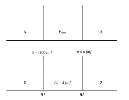
Fig. 11 Initial boundary conditions for the “fancy” race. (a) traffic flow (b) river flow.

Figure 11 represents the initial boundary conditions for both traffic (a) and river (b) flows. They define two Riemann problems at location \(x = -200 \mathrm{m}\) and \(x = 0 \mathrm{m}\). We are going to first focus on the front of the race, i.e., the Riemann problem at \(x = 0 \mathrm{m}\). Our first objective is to draw the space-time diagram in both cases. Figure 12 provides the fundamental diagram of the traffic flow.

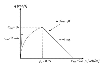
Fig. 12 The traffic fundamental diagram providing the model parameters

Question 1

The fundamental diagram in Figure 12 is quadratic in free-flow and linear in congestion. The equations are

\[\begin{split} \begin{align} Q(\rho) &= a \rho^2 + b\rho \quad &&\text{in free-flow} \\ Q(\rho) &= w(\rho_{max} - \rho) \quad &&\text{in congestion} \end{align} \end{split}\]

Model answer

\(w\) is the slope of the line in congestion modus.

\[ w = \frac{q_{max} - 0}{\rho_{max} - \rho_c} = \frac{0.6}{0.02 - 0.05} = 4 \mathrm{m/s}\]

Model answer

To find the value of \(a\),

\(Q(\rho_c) = a \rho_c^2 + b\rho_c = q_{max}\)

\(a = \frac{q_{max} - v_{max}\rho_c}{\rho_c^2}= -20 \mathrm{m/s}\)

To find the value of \(b\),

\(Q'(0) = 2a \cdot 0 + b = v_{max}\)

Question 2

Draw the space-time diagram corresponding the Riemann problem at \(x = 0 \mathrm{m}\) considering that the traffic obeys to the LWR model (first order macroscopic traffic flow model - cf. lecture 14). You will need it to answer the following questions.

Model Answer

You should have drawn a rarefaction wave to represent the front of the race (downstream \(x=0\)), otherwise double-check lecture 14.

Model Answer

The speed is the slope of the \(q\)-\(\rho\) diagram. Have a look at the first part.

The steepest part of the curve is when \(\rho = 0\) and the most gentle part when \(\rho = \rho_c\). The fastest kinematic wave speed is \(13 \mathrm{m/s}\) (\(v_{max}\)). The slowest kinematic wave speed is \(Q'(\rho_c) = 2 a \rho_c + v_{max} = 11 \mathrm{m/s}\)

Draw the final space-time diagram with all the relevant information.

Model Answer

Your space-time diagram should match the following:

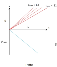
Fig. 13 Space-Time Diagram for Traffic

Question 3

Let’s consider we have a referee waiting for the race at \(x = 200 \mathrm{m}\) (she will wait for the water flow too later on!).

Model Answer

The first car follows the fastest wave while the pack arrives right after the slowest wave. Front wave arrives at

\[ t_1 = \frac{200 \mathrm{m}}{v_{max}} = 15.4 \mathrm{s} \]

Model Answer

The first car follows the fastest wave while the pack arrives right after the slowest wave.

The main pack arrives at

\[ t_2 = \frac{200}{11} = 18.2 \mathrm{s} \]

Question 4

Model Answer

We look for the kinematic wave starting at \(x = 0\) at \(t = 0\) and reaching \(x = 200\) at \(t\). The slope of this kinematic wave is \(Q'(\rho)\) but also \(\frac{x}{t}\).

So,

\[2a\rho + v_{max} = \frac{x}{t}\]

Hence,

\[\rho = \frac{\frac{x}{t} - v_{max}}{2a}\]

Question 5

Model Answer

The condition is when the integral of the flow at \(x = 200 \mathrm{m}\) is equal to \(1\).

Model Answer

The conservation principle makes the calculation straightforward as we have

\[ \rho_c (x - 0) = 0 + q_{max}T - 1 \]

So,

\[ T = \frac{1 + k_c x}{q_{max}} = 18.33 > t_2 \]

Question 6

Draw now the space-time diagram corresponding to the Riemann problem at \(x = 0 \mathrm{m}\) for the river flow. Please refer to the non-linear solution method in lecture 15. Remember that a python code has been provided to automatically determine the state diagram, so you only have to draw the space-time diagram. Do not use the linear approximation here, as the initial conidition is too sharp.

Model Answer

\[d_m = 0.56 \mathrm{m}\]

\[ V = 4.08 \mathrm{m/s} \]

(this only requires to set the values in the code Water_flow and run it)

Question 7

Question 8

Question 9

Model Answer

For a rarefaction wave, wave speeds are defined by \(\lambda_1(U)\) where, \(U\) is between the two boundary states (here \(U_{l}\) and \(U_m\)). The kinematic wave speeds are \(\lambda(U_l)\) and \(\lambda(U_m)\) with \(\lambda = V - \sqrt{gd}\).

Question 10

Model Answer

For a shockwave, the speed is given by the Rankine-Hugoniot condition, which depends on the two boundary states (here \(U_m\) and \(U_r\)).

This wave is a shockwave, whose speed is

\[ \frac{U_r d_r - U_m d_m}{d_r - d_m} = 4.1 \mathrm{m/s} \]

Question 11

Model Answer

Use the speed of the front wave from the previous question:

\[ v = 4.1 m/s \]

\[ t= \frac{s}{v} = \frac{200}{4.1} = 48.8 \mathrm{s}\]

Model Answer

After the cars, see question 3 (first car arrives at \(t = 15.4 \mathrm{s}\)).

Question 12

Model Answer

A linear diagram is free-flow with a free-flow speed equal to \(4.1 \mathrm{m/s}\). Because the front wave in water is a single wave. The only way to get that with the traffic is that the fan collapses into a signgle contact wave, which can only happen in the fundamental diagram in linear in free-flow.

Model Answer

With the linearization, the state diagram is a simple triangle, whose base is \((0, 0)\), \((d_0, 0)\). The height of this triangle represents the speed at \(U_m\), which is also the speed of the shockwave in that particular case as the downstream state is \((0, 0)\). The slope of the triangle is \(\sqrt{\frac{2d}{d_0}}\).

In this end, we want that :

\[ \sqrt{\frac{2g}{d_0}} \cdot \frac{d_0}{2} = \sqrt{\frac{gd_0}{2}} > 13 = v_{max, traffic} \]

It happens when \(d_0 > 34.34 \mathrm{m}\). Note that when you check with the non-linear state diagram, the value is different close to \(18 \mathrm{m}\) because it is clear that non-linear effect matters here.

Question 13

Now we focus on the rear Riemann problem at \(x = -200 \mathrm{m}\).

Model Answer

A steady shockwave whose speed is \(0\). Physically, that means that even if now cars are allowed to drive backwards, they don’t!

Question 14

Model Answer

Because the eigenvalues of the river flow problem are symmetric when \(V = 0 (\lambda = \pm \sqrt{gh})\), the solutions are also symmetric if the initial condition is. So, it suffices to reverse the solution of the front Riemann problem to derive the rear Riemann problem.

Question 15

Model Answer

It is when the contact wave propagating backward from \(x = 0\) (see the solution of the front Riemann problem in Q2) meets the steady shockwave of the rear Riemann problem. The first wave starts at \(x = 0, t = 0\) with a speed \(-4 \mathrm{m/s}\) (see Figure 12 and question Q1) and the second from \(x = -200\) at \(t = 0\), with a speed equal to \(0\). They meet at time \(t = 50 \mathrm{s}\).

Question 16

Model Answer

There are two boundary waves starting at \(x = 0 \mathrm{m}\) and \(x = -200 \mathrm{m}\) have a speed equal to \(-4.4\) and \(4.4 \mathrm{m/s}\) respectively. So, they meet at time \(22.7 \mathrm{s}\). It is worth noticing that the initial state disappears quicker in the river (water is less “stable” than a compact car platoon!)

\[\begin{split} \begin{align} -4.4 \cdot t &= -200 + 4.4 \cdot t \\ 8.8 \cdot t &= 200 \\ t &= 22.7 \mathrm{s} \end{align} \end{split}\]