CIE_4140_Lecture_2_2_Python

Vibration of 1 DOF system without damping under harmonic excitation

import sympy as sp

u = sp.symbols('u',cls=sp.Function)
t, omega_0, F_0, m, omega = sp.symbols('t, omega_0, F_0, m, omega',real=True,positive=True)
u_0, v_0 = sp.symbols('u_0, v_0')

Equation of motion

Equation_of_Motion= sp.Eq(sp.diff(u(t),t,2)+omega_0 **2 * u(t),F_0*sp.cos(omega*t)/m)
display(Equation_of_Motion)

\[\displaystyle \omega_{0}^{2} u{\left(t \right)} + \frac{d^{2}}{d t^{2}} u{\left(t \right)} = \frac{F_{0} \cos{\left(\omega t \right)}}{m}\]

Solution of the equation of motion with inital displacement \(x_0\) and initial velocity \(v_0\)

u_sol = sp.dsolve(Equation_of_Motion, u(t), ics={u(0): u_0 , u(t).diff(t , 1).subs(t , 0) : v_0}).rhs
display(u_sol)

\[\displaystyle - \frac{F_{0} \cos{\left(\omega t \right)}}{m \left(\omega^{2} - \omega_{0}^{2}\right)} + \frac{\left(F_{0} + m \omega^{2} u_{0} - m \omega_{0}^{2} u_{0}\right) \cos{\left(\omega_{0} t \right)}}{m \omega^{2} - m \omega_{0}^{2}} + \frac{v_{0} \sin{\left(\omega_{0} t \right)}}{\omega_{0}}\]

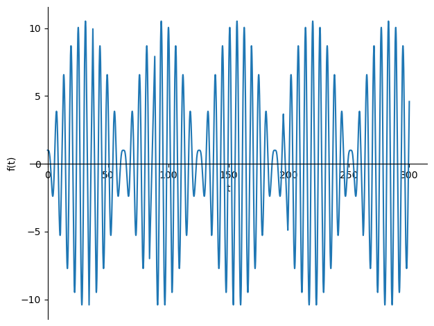
The phenomenon of beating

sp.plot(u_sol.subs([(u_0,1),(v_0,0),(F_0,1),(m,1),(omega_0,1),(omega,1.1)]),(t,0,300));

%matplotlib notebook

import numpy as np
import matplotlib.pyplot as plt
from matplotlib.animation import FuncAnimation

u_func = sp.lambdify((u_0,v_0,F_0,m,omega_0,omega,t),u_sol)

fig, ax = plt.subplots()
tdata = np.linspace(0,300,500)
line, = ax.plot([], [])
ax.set_xlim(0, 300)
ax.set_ylim(-10, 10)

def update(frame):
    ydata = u_func(u_0=1,v_0=0,F_0=1,m=1,omega_0=1,omega=frame,t=tdata)
    ax.set_title("Displacement versus time for $\omega$ = "+str(np.round(frame,2)))
    line.set_data(tdata, ydata)

ani = FuncAnimation(fig, update, frames=np.linspace(1.1,1.6,100),interval = 100)
plt.show()

Forced Vibration of 1 DOF system without damping under harmonic excitation

Equation of motion

display(Equation_of_Motion)

\[\displaystyle \omega_{0}^{2} u{\left(t \right)} + \frac{d^{2}}{d t^{2}} u{\left(t \right)} = \frac{F_{0} \cos{\left(\omega t \right)}}{m}\]

The steady-state solution should be sought for in the form \(x(t) = Xcos(\omega*t)\) The equation with respect to the amplitude of the steady-state vibration:

U = sp.symbols('U')
Equation_for_amplitude_of_u_steady = sp.simplify(Equation_of_Motion.subs(u(t), U*sp.cos(omega*t)))
Equation_for_amplitude_of_u_steady = sp.Eq(Equation_for_amplitude_of_u_steady.lhs * m / sp.cos(omega*t),
                                           Equation_for_amplitude_of_u_steady.rhs * m / sp.cos(omega*t))
display(sp.simplify(Equation_for_amplitude_of_u_steady))

\[\displaystyle F_{0} = U m \left(- \omega^{2} + \omega_{0}^{2}\right)\]

Amplitude of the steady-state vibration

U_steady = sp.solve(Equation_for_amplitude_of_u_steady, U)[0]
display(U_steady)

\[\displaystyle - \frac{F_{0}}{m \left(\omega^{2} - \omega_{0}^{2}\right)}\]

Frequency dependence of the amplitude:

sp.plot(U_steady.subs([(F_0,1),(m,1),(omega_0,1)]), (omega , 0 , 3), ylim = [-5 , 5]);

Development of resonance in time

Equation of Motion

display(Equation_of_Motion)

\[\displaystyle \omega_{0}^{2} u{\left(t \right)} + \frac{d^{2}}{d t^{2}} u{\left(t \right)} = \frac{F_{0} \cos{\left(\omega t \right)}}{m}\]

Solution of the equation of motion with inital displacement \(x_0\) and initial velocity \(v_0\)

u_sol = sp.dsolve(Equation_of_Motion, u(t), ics={u(0): u_0 , u(t).diff(t , 1).subs(t , 0) : v_0}).rhs
display(u_sol)

\[\displaystyle - \frac{F_{0} \cos{\left(\omega t \right)}}{m \left(\omega^{2} - \omega_{0}^{2}\right)} + \frac{\left(F_{0} + m \omega^{2} u_{0} - m \omega_{0}^{2} u_{0}\right) \cos{\left(\omega_{0} t \right)}}{m \omega^{2} - m \omega_{0}^{2}} + \frac{v_{0} \sin{\left(\omega_{0} t \right)}}{\omega_{0}}\]

Development of resonance from zero initial conditions

displacement_in_resonance = sp.limit(u_sol.subs([(u_0,0),(v_0,0)]),omega_0,omega)
display(displacement_in_resonance)

\[\displaystyle \frac{F_{0} t \sin{\left(\omega t \right)}}{2 m \omega}\]

sp.plot(displacement_in_resonance.subs([(F_0,1),(m,1),(omega,1)]), (t , 0 , 50));

displacement_in_resonance_func = sp.lambdify((F_0,m,omega,t),displacement_in_resonance)

fig, ax = plt.subplots()
tdata = np.linspace(0,50,500)
line, = ax.plot([], [])
ax.set_xlim(0, 50)
ax.set_ylim(-50, 50)

def update(frame):
    ydata = displacement_in_resonance_func(F_0=1, m=1, omega = frame, t = tdata)
    ax.set_title("resonance development at different frequencies for $\omega$ = "+str(np.round(frame,2)))
    line.set_data(tdata, ydata)

ani = FuncAnimation(fig, update, frames=np.linspace(0.5,1.5,100),interval = 100)
plt.show()

Variation of the energy in time

Energy =m/2*sp.diff(u_sol,t)**2 + m/2*omega_0**2*u_sol**2
display(Energy)

\[\displaystyle \frac{m \omega_{0}^{2} \left(- \frac{F_{0} \cos{\left(\omega t \right)}}{m \left(\omega^{2} - \omega_{0}^{2}\right)} + \frac{\left(F_{0} + m \omega^{2} u_{0} - m \omega_{0}^{2} u_{0}\right) \cos{\left(\omega_{0} t \right)}}{m \omega^{2} - m \omega_{0}^{2}} + \frac{v_{0} \sin{\left(\omega_{0} t \right)}}{\omega_{0}}\right)^{2}}{2} + \frac{m \left(\frac{F_{0} \omega \sin{\left(\omega t \right)}}{m \left(\omega^{2} - \omega_{0}^{2}\right)} - \frac{\omega_{0} \left(F_{0} + m \omega^{2} u_{0} - m \omega_{0}^{2} u_{0}\right) \sin{\left(\omega_{0} t \right)}}{m \omega^{2} - m \omega_{0}^{2}} + v_{0} \cos{\left(\omega_{0} t \right)}\right)^{2}}{2}\]

sp.plot(Energy.subs([(u_0,1),(v_0,0),(F_0,1),(m,1),(omega_0,1),(omega,1.1)]), (t , 0 , 300));

Energy_func = sp.lambdify((u_0,v_0,F_0,m,omega_0,omega,t),Energy)

fig, ax = plt.subplots()
tdata = np.linspace(0,300,500)
line, = ax.plot([], [])
ax.set_xlim(0, 300)
ax.set_ylim(0, 60)

def update(frame):
    ydata = Energy_func(u_0=1,v_0=0,F_0=1,m=1,omega=frame,omega_0=1,t=tdata)
    ax.set_title("Energy versus time for $\omega$ = "+str(np.round(frame,2)))
    line.set_data(tdata, ydata)

ani = FuncAnimation(fig, update, frames=np.linspace(1.1,1.6,100),interval = 100)
plt.show()